


Probability with Engineering Applications
Topics studied in previous class
•Sampling without replacement and its
relation to random samples
•Sample spaces with countably infinite
outcomes
•Axiom III for countably infinite disjoint sets
•Relative frequencies; many trials
•Uncountably infinite sample spaces
•Real numbers versus reality
Measurements are rational
•A physical measurement made with an
instrument yields a rational number
•At the microscopic level, most physical
phenomena are discrete
•Any electrical charge is an integer multiple
of the electrical charge of an electron
•Electrical current (charge/unit time) is a
rational multiple of the quantity
one electron charge/s
But, the models are real numbers
•The real numbers in computer programs
are actually rational numbers — irrational
numbers cannot be represented exactly
•Then, why are physical parameters
modeled as continuous variables?
•Easier to get (the “right”) answers
•Calculus can be used:
 assumes that i is a continuous function of t
Measurements versus models
•All actual measurements result in rational
numbers, but we model the measurement
as being an arbitrary real number
•We all understand that V = 1.235 volts
really means that V is some real number in
the range 1.2345 ≤ V ≤
1.2355 volts
•This modeling is useful and convenient in
the physical sciences and engineering
but causes difficulties in probability theory
Real numbers in probability
•Uncountably infinite sample spaces are
the real line (or intervals thereof )
•Such spaces cause subtle mathematical
difficulties in probability theory
•The resolution of these difficulties led to
the development of the axiomatic theory of
probability
•We will look only at the end results, not the
gory details
Relative frequencies converge to 0
•The output of rand() is a good model
for repeated trials for the experiment of
picking a number at random in (0, 1)
•Every call to rand() returns a different
number
•Relative frequency of a specific number in
(0,1) converges to 0
•Actually, the output of rand() is periodic
(with long period,) and the numbers will repeat
P{outcome} is always 0
•The only model that works for uncountably
infinite sample spaces is for each outcome
to have probability 0
•But, on each trial, some outcome occurs
•Moral: An event whose probability is zero
can occur
•Complementary event has probability one
•Immoral: An event whose probability is
one need not occur on every trial!
Events of probability zero
•A event of probability zero is one to which
we assign a probability of 0
•A event of probability zero is not the same
as
 , the impossible event
•A zero-probability event can occur on a
trial of the experiment:
never ever does
•It is just that a zero-probability event does
not occur too often — in fact, it is usually
observed only once at most
Events of probability one
•The complement of an event of probability
zero is called an event of probability one
•An event of probability one is not the same
as
 , the certain or sure event
•An event of probability one need not occur
on every trial:
occurs on all trials
•An event of probability one is called an
almost sure event because it almost
always occurs
Any probabilities other than 0 or 1?
•If every outcome is an event of probability
zero, then isn’t it true that any event A
must also have probability zero?
•P(A) = sum of the probabilities of all the
outcomes that comprise A
= 0 + 0 + … = 0?
•No, the above is a mis-application of
Axiom III (which applies to countable
unions only)
P(countable event) = 0
•Since each outcome has probability zero,
a countable event, that is, an event that
has a countable number of outcomes, also
has probability zero (by Axiom III)
•Axiom III does not say that the probability
of an uncountable event is the sum of the
probabilities of the outcomes
•The nonzero (and non-one) probabilities
are assigned to such uncountable events
A probability paradox
•Example: Choose a random number
between 0 and 1
•The rational numbers between 0 and 1 are
a countable set
•P(outcome is a rational number) = 0
•But, in any simulation of this experiment,
e.g. via calls to rand(), the “outcome”
will be a rational number
•Remember that rand()is a model
Intervals are uncountable events
•Example: Choose a random number
between 0 and 1
•Each outcome (and also any countable set
of outcomes) has probability zero
•However, P{a < outcome < b} = b – a
for 0 ≤ a < b ≤ 1
•The nonzero probabilities are assigned to
the intervals of the line, not to outcomes!
Asking the right question
•In most physical applications, the question
“Does x = 0.213482774099070267623…?”
is meaningless
•If x were 0.213482774099070267624…
instead, the airplane will still fly, the bridge
will still stand, the modem will still connect
l In most instances, we are satisfied if x is in
some specified range (design specs)
•“Does x ∈(a,b)?” is the right question!
Intervals have nonzero probabilities
•Example: Choose a random number
between 0 and 1
•P{a < outcome < b} = b–a for 0 ≤ a < b
≤ 1
•P{0.4 < outcome < 0.6} = 0.2
•N calls to rand() give N numbers,
roughly 20% of which are in the interval
(0.4, 0.6)
•At most one (and most likely none!) of
these will be 0.57689231
What about P(arbitrary subset)?
•For uncountably infinite sample spaces, a
consistent probability assignment to all the
subsets of
 is not possible
•If we restrict the class of subsets of
 to
to
which we will assign probabilities, then a
consistent assignment of probabilities is
possible
•It is meaningless to talk of probabilities of
subsets that are not in this restricted class
Rules for collections of events
•Let
 denote the collection of subsets of

that we will call the events and to which
we will assign probabilities
•The members of
 are subsets of

•Rule I:
•Rule II: If
 also
also
•Rule III: If
 is a
is a
countable sequence of events, then,
 also
also
The
 field of events
•A collection
 of subsets of
 that satisfies
Rules I–III is called a

•Rules I–III can be summarized as follows:
A field contains
 and is closed under
complementation and countable unions
•“Closed under” means the result of the
specified operation also belongs to

•By DeMorgan’s theorem, the field is also
closed under countable intersections
Small
fields
•For a finite or countably infinite sample
space, the collection of all the subsets of
 is a
field
is a
field
•If
 ,
this field has
,
this field has
 events in it
•Smaller
fields
also exist:
 is a
field
as is
is a
field
as is

•Given any partition of
 ,
the collection of
,
the collection of
all the sets that can be written as the union
of the sets in the partition is also a
field
The
field of the real line
•When
is the real line (or an interval
thereof), we have a Rule IV for the field
•Rule IV: The field contains all intervals
of the form (a, b) with a < b
•It can be shown that Rules I–III imply that
intervals of the form

also belong to the field
More on the field of the real line
•The field of the real line contains all
intervals of all types (open, closed etc)
•Since we will assign probabilities only to
the members of the field, this ensures
that all the right engineering questions
such as
“What is P{0.23 < outcome < 0.25}?”
“What is P{0.23 ≤ outcome ≤
0.29}?”
have useful answers
Not in the field of the real line?
•The field of the real line contains all the
intervals of all types
•It contains the complements and the
countable unions and intersections of
these intervals
•Are there subsets of the real line that are
not of this type? Yes
•Professor, can you describe one to us?
•Need Math 441 to understand description
The Probability Space
•The probability space is the formal
statement of the axiomatic theory
•A probability space
 consists of
nthe sample spaceconsisting of all
possible outcomes of the experiment
nthe
 of events which includes all
of the interesting subsets of Ω
nthe probability measure P(•) that assigns
probabilities to the events in

The Probability Space (continued)
•The probability measure P(•) assigns
probabilities to the events in
 subject to
the following rules (axioms)
•Axiom I: for all events A
•Axiom II:

•Axiom III: If is a
is a
countable sequence of disjoint events,
then


Footnote to Probability Space
•Ifis the real line, then we assume that
, the field of events, consists of all the
open intervals, and all the other events
that it must contain as per Rules I–III
•In this case, also contains all semiclosed
and closed intervals as well
•There do exist weird subsets ofthat are
not in and do not have probabilities
•These subsets never arise in applications
Duh! So what is all this good for?
•The axiomatic approach is the foundation
•The consequences of the axioms have
already been looked at earlier
•In practice, the formal axiomatic approach
to probability is not used on a everyday
basis in solving problems
•It is important to know what are the right
questions to ask: In infinite sample spaces,
ask for P{a < x < b} and not for P{x = c}
We know everything already
•The axiomatic theory tells about the
probability measure P(•)
•Since we know P(•), what is left to study?
•Generally, P(•) is known for only some of
the events
•The probability calculus allows us to
calculate the probabilities of other events
•So, why don’t we estimate these other
probabilities via (say) relative frequencies?
We don’t know everything already
•So, why don’t we estimate these other
probabilities via (say) relative frequencies?
•Some probabilities may be too expensive
or too small to estimate
•reliability of complex systems is more easily
calculated than measured
•how do we measure the probability that a
nuclear reactor has a meltdown?
•Calculate probabilities of complex events
from probabilities of simpler events
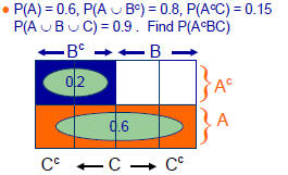
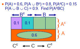
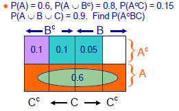
An example
•Example: Events A, B, C are defined on a
sample space W. Given that P(A) = 0.6,
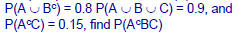
•As before, the first step is to draw a
Karnaugh map
Find P(AcBC)
Find P(AcBC)
Find P(AcBC)
Summary
•We discussed measurements vs models
•We studied uncountably infinite sample
spaces and noted P{outcome} = 0
•We discussed the restricted notion of
events in uncountably infinite sample
spaces
•We gave a formal statement of the
concept of a probability space
•We did an example